15.1 Constraints
In our development thus far, we have assumed that a dataset can be any set of factoids. This is rarely the case. Usually, there are constraints that limit the set of possibilities. Not every set of facts about parenthood is possible, e.g. a person cannot be his own parent.
In many database texts, constraints are written in direct form; they say what must be true. For example, if an entity appears as the first argument of a fact involving the father relation, it must also appear in the male relation.
In what follows, we use a slightly less direct approach; we say what must not be true. To do this, we use a special 0-ary relation, here called illegal; and we define it to be true in any extension that does not satisfy our constraints.
This approach works particularly well for consistency constraints like the one stating that a person cannot be his own parent.
It also works well for mutual exclusion constraints like the one below, which states that a person cannot be in both the male and the female relations.
| illegal :- male(X) & female(X) |
Using this technique, we can also write the inclusion dependency mentioned earlier. There is an error if an entity is the first argument of a factoid involving the father predicate and it does not occur in a factoid involving the male predicate.
| illegal :- father(X,Y) & ~male(X) |
Database management systems can use such constraints in a variety of ways. They can be used to optimize the processing of queries. They can also be used to check that updates do not lead to unacceptable extensions. In this chapter, we discuss some of these uses.
15.2 Alerting
Rejecting inconsistent datasets is essential in some applications. However, simply reporting that there are failures is not as useful as pinpointing the violated constraints so that the programmer or user can modify his datasets accordingly.
One way of providing such information is to replace ordinary constraints with annotated constraints. An annotated constraint is similar to an ordinary constraint, except that, in place of the boolean constant illegal, the head of the constraint is an atom with an appropriate relation constant (e.g. warning) applied to a message to be transmitted to the user in the event that the body evaluates to true (i.e. the corresponding constraint is violated.)
For example, we could rewrite the non-reflexivity and the antisymmetry constraints on the parent relation with the annotated constraint shown below, and our execution system could use constraints like these to generate warning messages for the user.
| warning("People cannot be their own parents.") :- parent(X,X) |
| warning("Parenthood is antisymmetric.") :- parent(X,Y) & parent(Y,Z) |
Since constraints are simply rules, we can make such annotated constraints more informative by constructing messages that give information about specific instances of the problem.
For example, the following annotated constraint constructs a separate message for each violation of the non-reflexivity condition.
warning(Msg) :-
parent(X,X) &
stringify(X,XS) &
stringappend(XS," cannot be his own parent.",Msg)
|
15.3 Conflict Sets
Alerting the user to the nature of a problem is better than simply reporting that a problem exists. However, and even better way of dealing with inconsistency is to identify the specific data set facts responsible for an inconsistency. Each such set of facts is called a conflict set.
As an example, consider the constraints shown below.
| illegal :- p(a) & q(a) |
| illegal :- ~q(a) & r(a) |
Now suppose we have the following dataset.
Note that, in general, there can be more than one conflict set responsible for a given constraint violation. As an example, consider the constraint shown on the left below and the dataset shown on the right.
| illegal :- p(a) & q(a) |
| illegal :- ~q(a) & r(a) |
In some cases, there can be infinitely many ground conflict sets. Problem solved by allowing for conflict sets with atoms that contain variables.
Computing conflict sets. One way for a system to do this is to collect the base facts used in determining that a dataset is inconsistent with a set of constraints. If there is more than one way that a dataset is inconsistent, then it is desirable to compute the set of of all such derivations.
15.4 Dataset Repair
We can think of the set of justifications for the illegal relation as a disjunction of conjunctions. illegal is true if and only if any of the conjunctions is true.
To repair an inconsistent dataset, we need to reverse the truth value of at least one conjunct in every conflict set.
In general, finding a minimal repair requires significant amount of search.
Unfortunately, getting to a consistent dataset is not as simple as reversing one factoid from each justification. If we change the truth value of a factoid, this can lead to new inconsistencies. To see how this can happen, consider the following example.
| illegal :- p(a) & q(a) |
| illegal :- ~q(a) & r(a) |
Now suppose we have the dataset shown below.
This dataset violates the first constraint above. If were to try to repair this problem by deleting q(a), the resulting dataset would then violate the second constraint.
In general, it may be necessary to try a sequence of repairs to find one that works. The downside of this is that, in so doing, one can get lost in the process.
Luckily, there is a method sometimes helps in this regard. In general, it is possible to offer the user a set of changes that guarantees that he can reach a consistent dataset without backing up. The trick is to compute consequences of constraints and to use those consequences in computing repair sets. If one then executes one of the resulting repairs, he knows that he can reach a consistent dataset without reversing that decision.
In the case, we just examined, it is possible to deduce an additional constraint from the two original constraints. See below.
| illegal :- p(a) & q(a) |
| illegal :- ~q(a) & r(a) |
| illegal :- p(a) & r(a) |
In this case, our dataset would yield the following problems.
In this case, changing q(a) does not fix all of these problems and hence that suggestion would be rejected in favor of changing p(a).
15.5 Constraint Satisfaction
In the preceding sections, we showed how to check whether a given dataset satisfies a set of constraints, and we showed how to deal with a dataset that violates our constraints. In this section and the sections that follow, we are given constraints but no datasets, and our job is to construct a dataset that satisfies the given constraints.
The process of finding a dataset that satisfies a set of constraints is often called logical constraint satisfaction or, more simply, constraint satisfaction (though that phrase is often used to describe a generalization of logical constraint satisfaction). It is closely related to the process of determining the satisfiability of a set of constraints. The main difference is that in logical constraint satisfaction we actually want a dataset whereas in satisfiability checking we are concerned only with the question of whether such a dataset exists. The distinction is of little importance since most satisfiability checking techniques work by constructing or attempting to construct datasets and so can be viewed as logical constraint satisfaction methods.
As an example of a logical constraint satisfaction problem, consider the task of coloring a planar map using only four colors, the idea being to assign each region a color so that no two adjacent regions are assigned the same color.
A typical map is shown below. There are six regions. Some are adjacent to each other, meaning that they cannot be assigned the same color. Others are not adjacent, meaning that they can be assigned the same color.
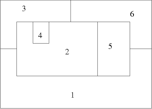
In what follows we use the symbols red, green, blue, purple, stand for the colors red, green, blue, and purple respectively.
To encode a coloring of the map, we use six unary relation constants r1, ..., r6, the idea being that one of these region relations holds of a color if and only if the region is assigned that color.
We want each region to be assigned at least one color. We can express this by defining a dataset to be illegal if any region relation does not hold of at least one color.
| illegal :- ~r1(red) & ~r1(green) & ~r1(blue) & ~r1(purple) |
| illegal :- ~r2(red) & ~r2(green) & ~r2(blue) & ~r2(purple) |
| illegal :- ~r3(red) & ~r3(green) & ~r3(blue) & ~r3(purple) |
| illegal :- ~r4(red) & ~r4(green) & ~r4(blue) & ~r4(purple) |
| illegal :- ~r5(red) & ~r5(green) & ~r5(blue) & ~r5(purple) |
| illegal :- ~r6(red) & ~r6(green) & ~r6(blue) & ~r6(purple) |
We also want each region to be assigned at most one color. We can formalize this constraint with the rules shown below. The first rule states that a dataset is illegal if r1 is true of a color C and a color D and if C and D are distinct.
| illegal :- r1(C) & r1(D) & distinct(C,D) |
| illegal :- r2(C) & r2(D) & distinct(C,D) |
| illegal :- r3(C) & r3(D) & distinct(C,D) |
| illegal :- r4(C) & r4(D) & distinct(C,D) |
| illegal :- r5(C) & r5(D) & distinct(C,D) |
| illegal :- r6(C) & r6(D) & distinct(C,D) |
Finally, Using our region relations, we can encode the adjacency constraints corresponding to our map as shown below. Since region 1 is adjacent to region 2 in the map, we say that a dataset is illegal if r1 and r2 are true of the same color. The remaining constraints capture the remaining adjacencies.
| illegal :- r1(C) & r2(C) |
| illegal :- r1(C) & r3(C) |
| illegal :- r1(C) & r5(C) |
| illegal :- r1(C) & r6(C) |
| illegal :- r2(C) & r3(C) |
| illegal :- r2(C) & r4(C) |
| illegal :- r2(C) & r5(C) |
| illegal :- r2(C) & r6(C) |
| illegal :- r3(C) & r4(C) |
| illegal :- r3(C) & r6(C) |
| illegal :- r5(C) & r6(C) |
In satisfiability checking, our job is to determine whether there is any dataset that satisfies these constraints; in logical constraint satisfaction, our job is to produce such a dataset if one exists.
15.6 Generate and Test
From a conceptual perspective, the simplest approach to solving a constraint satisfaction problem is Generate and Test. We generate candidate datasets and then test them to see whether any satisfies our constraints. If we find one that works, we are done; if none of the candidates works, we know that the constraints are unsatisfiable.
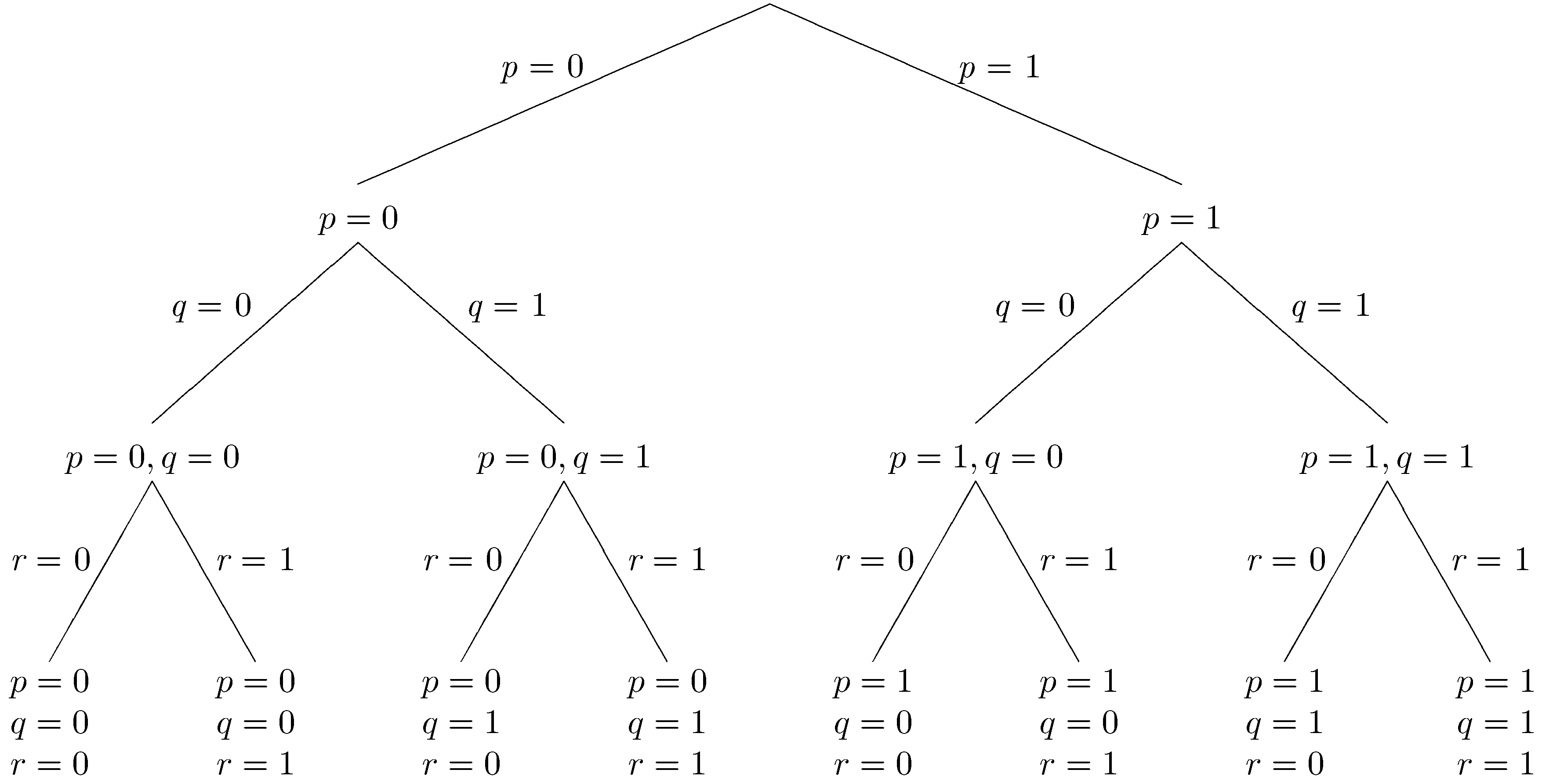
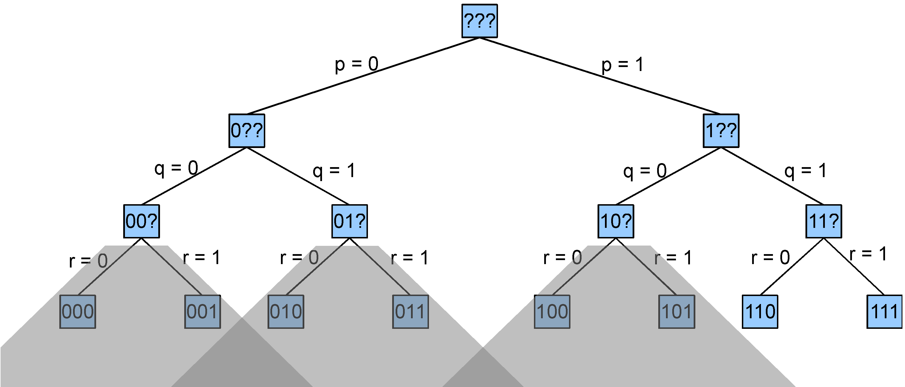
One way to generate candidate datasets systematically is to conceptualize the space of possibilities as a tree. Each node in the tree represents a partial or complete dataset and each branch represents a choice to include or exclude a factoid from the dataset. The fringe nodes of the tree represent complete datasets, where we have made decisions about every factoid.
The tree shown below is an example for a Herbrand base with just three factoids (p, q, and r). The eight fringe nodes correspond to the eight possible datasets. We have written p=0 here to mean that p is not in the dataset and p=1 to mean that p is in the dataset. So, the leftmost fringe node represents the empty dataset, and the rightmost fringe node represents the dataset consisting of all three factoids.
The main problem with Generate and Test is that the number of possible datasets can be very large. In this case, there are are only eight possibilities; but, for most problems, the set of possibilities is much larger. For example, there are 24 sentences in our map coloring example, and so there are 2^24 possible datasets. Generating all of those datasets can take a long time. Luckily, there are some ways that we can do better.
15.7 Backtracking Search
Backtracking search is a specialization of generate and test in which we interleave generation and testing. Here, we consider two varieties of backtracking search - complete dataset testing and partial dataset testing.
In complete dataset testing, we generate candidates systematically as in Generate and Test; but, instead of waiting to start testing until we have all candidates in hand, we test each complete dataset as it is generated. If the candidate satisfies our constraints, we are done. If not we "backtrack" and generate the next candidate. If we are lucky or if there are many candidates that work, this can lead to a reduction in computation time.
In the case of map coloring, this saves a significant amount of work. If we order our factoids systematically, first enumerating regions and then for each region enumerating colors, we find a dataset that satisfies our constraints after examining 8,116,191 possibilities, a significant reduction from the space of 16,777,216 possible datasets.
Partial dataset testing takes the idea of interleaving even farther. Rather than testing complete datasets, we test each partial dataset as it is generated to see whether it violates the constraints. Recognizing that a partial dataset does not work allows us to avoid generating the various completions of that partial dataset, and this can lead to significant savings.
Of course, there is additional cost in performing these extra tests. However, we know that the number of interior nodes in a binary tree is less than the number of fringe nodes. Consequently, the total number of tests in partial dataset testing is no more than double than the number of tests in complete dataset testing.
Consider once again our simple example with three factoids p, q, and r. Let's assume we have the constraints shown below.
| illegal :- ~p & ~q |
| illegal :- ~p & q |
| illegal :- p & ~q |
| illegal :- p & q & r |
| illegal :- p & ~r |
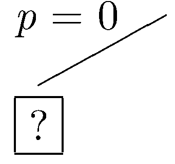
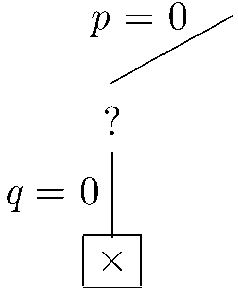
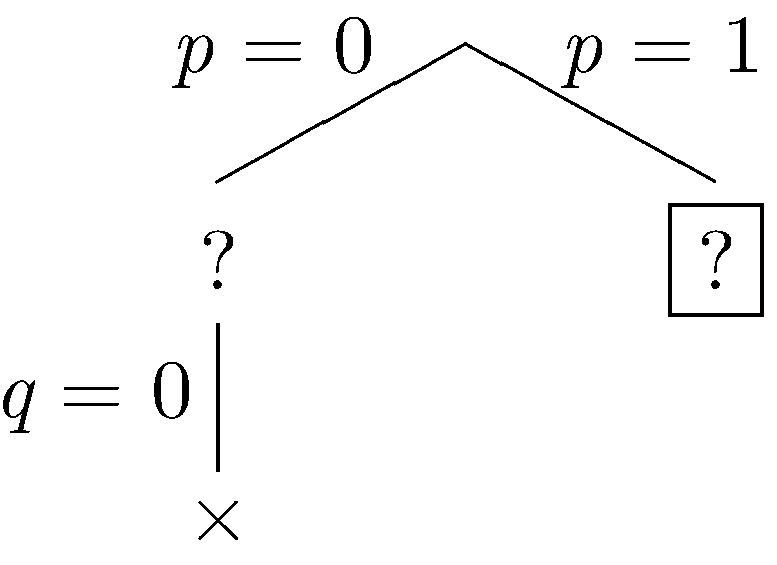
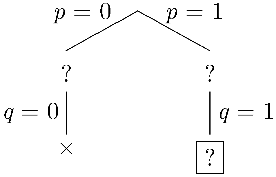
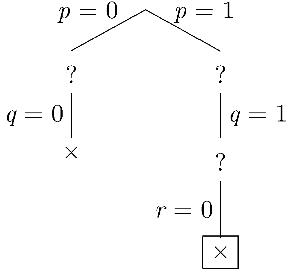
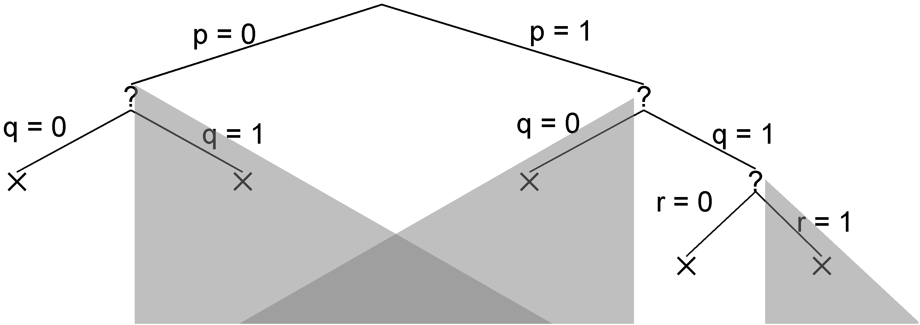
Now let's look at how partial dataset testing works in this case. At each step, we show the part of the tree explored so far. A boxed node is the current node. An × mark at a node indicates that the partial dataset at that node fails to satisfy at least one constraint. A ✓ indicates that the dataset at that node satisfies all of the constraints. A ? indicates that the partial dataset at the node neither satisfies nor fails to satisfy the constraints.
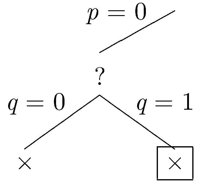
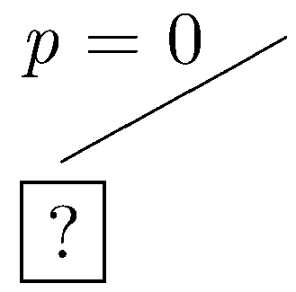
Let's start with the assumption that p is not in the dataset (i.e. p=0). This leads to the partial tree shown below.
Now, let's assume that q is not in the dataset. In this case, the partial dataset fails to satisfy the constraints, and the current branch is closed.
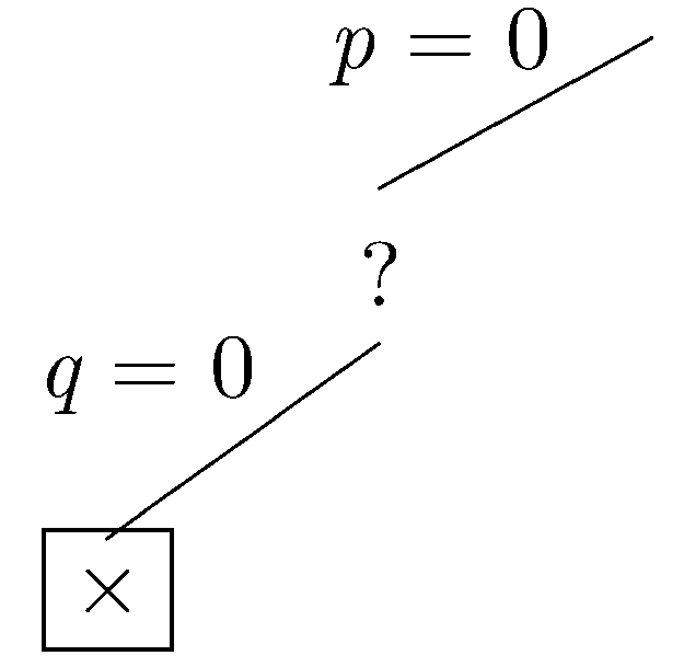
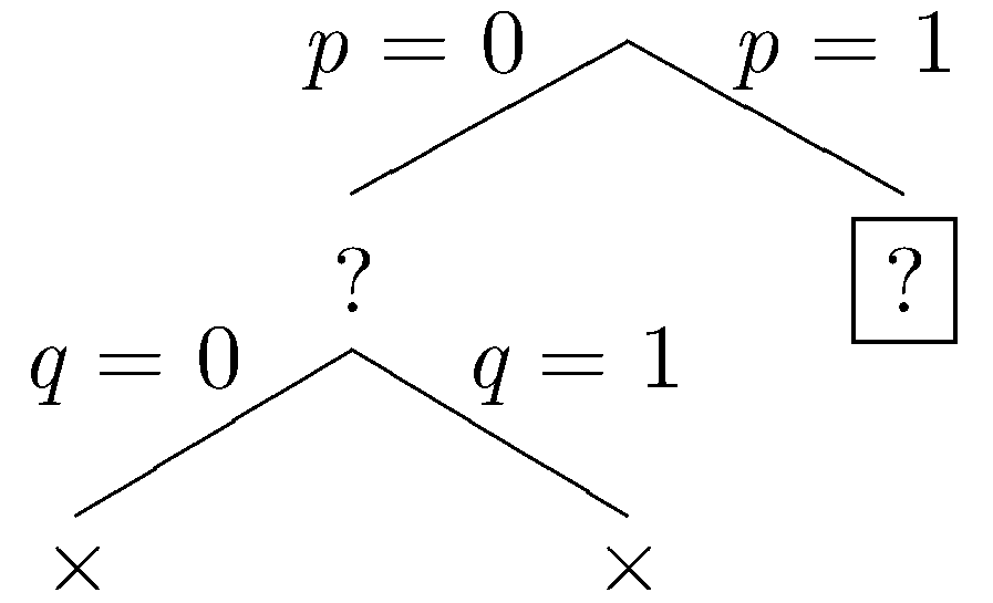
Since the current branch is closed, we backtrack to the most recent choice point where another branch can be taken. This time, let's assume that q is in the dataset.
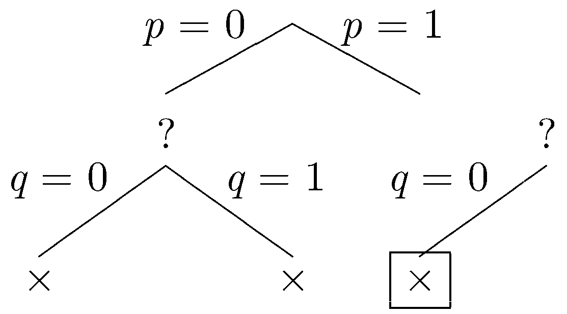
Again, the partial dataset fails to satisfy the constraints, and the current branch is closed. Again we backtrack to the most recent choice point where another branch can be taken. Let p be be in the dataset.
Let q be excluded.
Again, our the partial dataset fails to satisfy the constraints, and we backtrack. Let q be included.
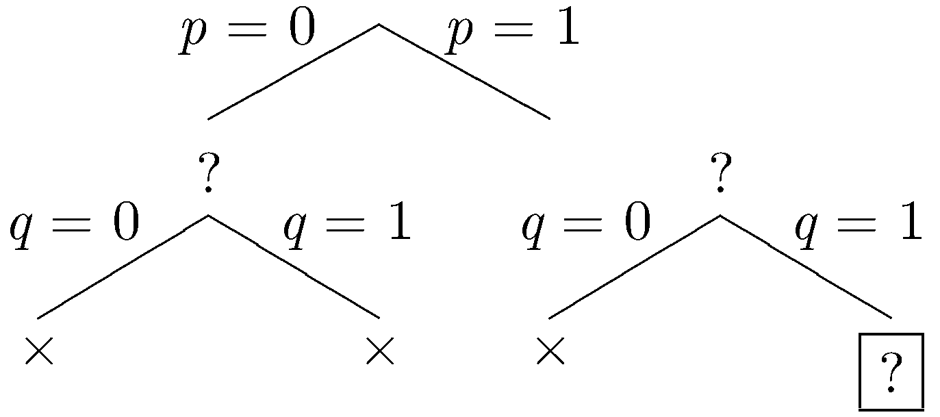
Let r be excluded.
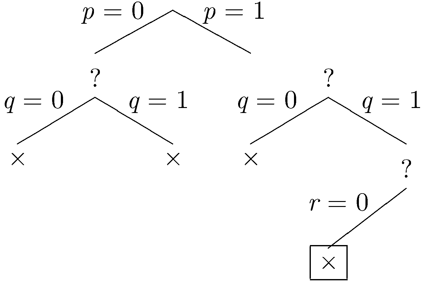
The constraints are violated by this dataset, and we backtrack one last time. Let r be inclued.
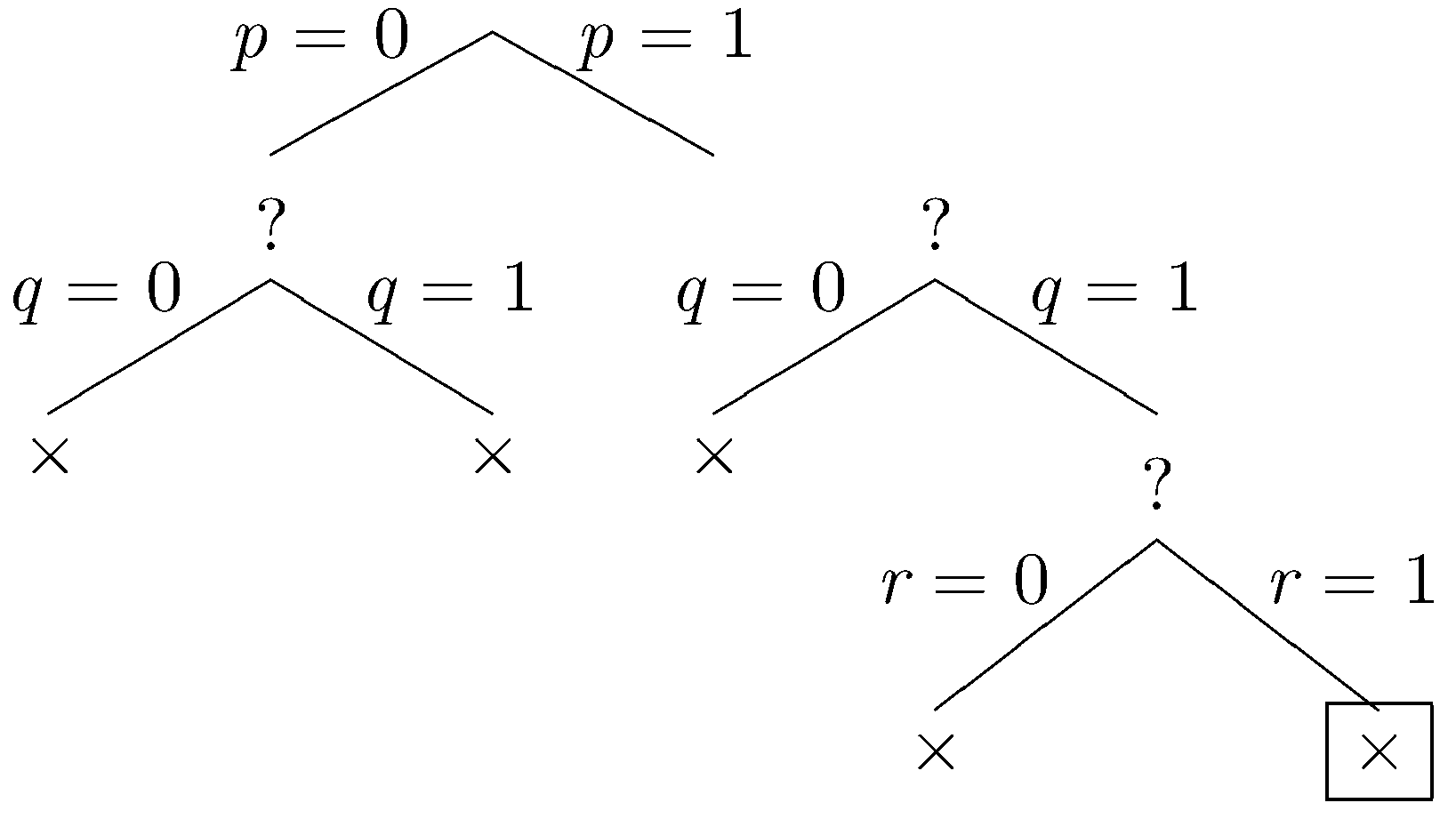
Once again, our constraints are violated. Since all branches have been explored and closed, the method determines that our constraints are unsatisfiable.
Looking at the full search tree compared to the portion explored by the basic backtracking search, we can see that the greyed out subtrees are all pruned from the search space. In this particular example, the savings are not spectacular. But in a bigger example with more propositions, the pruned subtrees can be much bigger.
The benefits of partial dataset testing are more significant in the case of our map coloring example. Using partial dataset testing, we can find a solution to the problem in a fraction of the time. In one test, finding a solution to the problem using complete dataset testing took 137 seconds whereas finding a solution using partial dataset testing took just 16 milliseconds.
15.8 DPLL
The Davis-Putnam-Logemann-Loveland method (DPLL) is a classic method for SAT solving. It is essentially backtracking search along with unit propagation (described below) and pure literal elimination (not described here). Most modern, logical constraint satisfaction systems are based on DPLL, with additional optimizations not discussed here.
A key step in DPLL is constraint simplification. As we decide whether to include or exclude a factoid from a dataset, there are opportunities to simplify our constraints to make them easier to test, to create additional opportunities for simplification, and to dictate choices for factoids we have not yet considered.
Suppose, for example, we have decided that p is in our dataset. (1) Each constraint containing ~p may be ignored because it must already be satisfied by the current partial dataset. (2) Each constraint containing a subgoal ~p may be modified (call the result φ') by removing from it all occurrences of the disjunct ¬p because, under all truth assignments where p has truth value 1, φ holds if and only if φ' holds.
If a proposition p has been assigned the truth value 0, we can simplify our sentences analogously. (1) Each disjunction containing a disjunct ¬p may be ignored because it must already be satisfied by the current partial assignment. (2) Each disjunction φ containing a disjunct p may be modified by removing from it all occurrences of the disjunct p.
Consider once again the example in the preceding section. If we include p in our dataset, we can simply our sentences as shown below. The first two sentences are dropped, and the literal p is dropped from the other three sentences.
| Original | | Simplified |
|---|
|
| illegal :- ~p & ~q | | − |
| illegal :- ~p & q | | − |
| illegal :- p & ~q | | illegal :- ~q |
| illegal :- p & q & r | | illegal :- q & r |
| illegal :- p & ~r | | illegal :- ~r |
While simplifying sentences is helpful in and of itself, the real value of simplification is that it enables further optimizations that can drastically decrease the search space.
One of these optimizations is unit propagation. In the course of the backtracking search, if we see a sentence that consists of single atom, say p, we know that the only possible satisfying assignments further down the branch must set p to true. In this case, we can fix p to be true and ignore the subbranch that sets p to false. Similarly, when we encounter a sentence that consists of a single negated atom, say ¬p, we can fix p to be false and ignore the other subbranch. This optimization is called unit propagation because sentences of the form p or ¬p are called units.
To see the benefits of this, let's redo example 1 with simplification and unit propagation. As we proceed through this example, we illustrate each step with the search tree on that step (on the left) and the simplified constraint set (in the table on the right).
To start, let's make p false.
 |
|
| Original | | Simplified |
|---|
|
| illegal :- ~p & ~q | | illegal :- ~q |
| illegal :- ~p & q | | illegal :- q |
| illegal :- p & ~q | | − |
| illegal :- p & q & r | | − |
| illegal :- p & ~r | | − |
|
In the simplified set of sentences, we have the unit ~q, so we fix q to be false (by unit propagation). (We also have the unit constraint q, so we could have fixed q to true. The result is the same in either case.)
 |
|
| Original | | Simplified |
|---|
|
| illegal :- ~p & ~q | | illegal |
| illegal :- ~p & q | | − |
| illegal :- p & ~q | | − |
| illegal :- p & q & r | | − |
| illegal :- p & ~r | | − |
|
Our constraints are falsified, so we backtrack to the most recent decision point, in this case all the way back at the root, and this time we let p be true.
 |
|
| Original | | Simplified |
|---|
|
| illegal :- ~p & ~q | | − |
| illegal :- ~p & q | | − |
| illegal :- p & ~q | | illegal :- ~q |
| illegal :- p & q & r | | illegal :- q & r |
| illegal :- p & ~r | | illegal :- ~r |
|
In the simplified set of sentences, we have the unit q so we do unit propagation, fixing q to be true. (We could also have performed unit propagation using the other unit r.)
 |
|
| Original | | Simplified |
|---|
|
| illegal :- ~p & ~q | | − |
| illegal :- ~p & q | | − |
| illegal :- p & ~q | | − |
| illegal :- p & q & r | | illegal :- r |
| illegal :- p & ~r | | illegal :- ~r |
|
In the simplified set of constraints, we have the unit ~r, so we do unit propagation, fixing r to be false.
 |
|
| Original | | Simplified |
|---|
|
| illegal :- ~p & ~q | | − |
| illegal :- ~p & q | | − |
| illegal :- p & ~q | | − |
| illegal :- p & q & r | | − |
| illegal :- p & ~r | | illegal |
|
Our constraints are violated on this branch, so the branch is closed. Since all branches are closed, the method determines that our constraints are unsatisfiable.
Compared to the tree explored by the backtracking search without unit propagation, we see that the greyed out subtrees are pruned away from the search space.
15.9 GSAT
Many practical SAT solvers based on complete search for models are routinely used to solve satisfiability problems of significant size. However, some problem instances are still impractical to solve using complete search for models.
In these problem instances, it is impractical to exhaustively eliminate every truth assignment as a possible model. In such situations, one may consider incomplete search methods - methods that answer correctly when they can but sometimes fail to answer. The basic idea is to sample a subset of truth assignments. If a satisfying assignment is found, then we can conclude that the input is satisfiable. If no satisfying assignment is found, then we don't know whether the input is satisfiable. In practice, modern incomplete SAT solvers tend to be very good at finding the satisfying assignments in a reasonable amount of time when they exist, but they still lack the ability to answer definitively that an input is unsatisfiable.
The first idea may be to uniformly sample a number of truth assignments from the space of all truth assignments. However, in large problem instances for with few satisfying assignments, one would expect to take a very long time before happening upon a satisfying assignment. What enables incomplete SAT solvers to work efficiently is the use of heuristics that frequently steer the search toward satisfying assignments. One family of incomplete SAT solvers uses local search heuristics to look for a truth assignment that maximizes the number of sentences it satisfies. Clearly, a set of sentences is satisfiable if and only if it is satisfied by an optimal truth assignment (optimal in terms of maximizing the number of sentences satisfied).
We look at one particular method called GSAT in more detail. The GSAT method starts with an arbitrary truth assignment. Then GSAT moves from one truth assignment to the next by flipping one of the propositions to achieve the greatest increase in the number of sentences satisfied. The search stops when it reaches a truth assignment such that the number of sentences satisfied cannot be increased by flipping the truth value of one proposition (in other words, a locally optimal point is reached).
Consider the set of constraints {illegal :- ~p & ~q &~r, illegal :- p, illegal :- q, illegal :- r}. This set of constraints is clearly unsatisfiable. What follows is one possible execution of GSAT on this case. For each step, we show the truth value for each factoid; we show whether constraint is satisfied or violated; and we show how many constraints are violated. In this case, we need this number to be 0 in order for the set as a whole to be satisfied. We start with an arbitrary assignment in which all factoids are true. (Note that, for space purposes here, we have written just the subgoals for each constraint. They are effectively violation conditions - if the condition is satisfied, it means the corresponding constraint is violated.)
| p |
q |
r |
|
~p & ~q & ~r |
p |
q |
r |
|
# violations |
| 1 |
1 |
1 |
|
0 |
1 |
1 |
1 |
|
3 |
Only one constraint is satisfied by this assignment. However, we can improve matters by flipping the value of p.
| p |
q |
r |
|
~p & ~q & ~r |
p |
q |
r |
|
# violations |
| 0 |
1 |
1 |
|
0 |
0 |
1 |
1 |
|
2 |
Still not satisfied, but we can improve matters by flipping the value of q.
| p |
q |
r |
|
~p & ~q & ~r |
p |
q |
r |
|
# violations |
| 0 |
0 |
1 |
|
0 |
0 |
0 |
1 |
|
1 |
Unfortunately, at this point, we are stuck. No flipping of a single proposition value can increase the number of sentences satisfied. The search terminates, suggesting that the our sentences are unsatisfiable.
Now, let's see what happens when we apply the method to a set or sentences that is satisfiable. Our set in this case is {illegal :- ~p, illegal :- p & ~q, illegal :- p & & ~r}. Let's say we start with a truth assignment in p is true and q and r are false. In this case, there are two violations.
| p |
q |
r |
|
~p |
p & ~q |
p & ~r |
|
# violations |
| 1 |
0 |
0 |
|
0 |
1 |
1 |
|
2 |
Flipping the value of q can improve matters.
| p |
q |
r |
|
~p |
p & ~q |
p & ~r |
|
# violations |
| 1 |
1 |
0 |
|
0 |
0 |
1 |
|
1 |
Flipping the value of r can improve matters further.
| p |
q |
r |
|
~p |
p & ~q |
p & ~r |
|
# violations |
| 1 |
1 |
1 |
|
0 |
0 |
0 |
|
0 |
Since all three sentences are satisfied, the set as a whole is satisfied. The search terminates, concluding that the set is satisfiable.
Unfortunately, local search of this sort is not guaranteed to be complete - the search may terminate without finding a satisfying assignment even though one exists. Depending on the starting assignment and the arbitrary choices in breaking ties between flipping one proposition vs another, the GSAT method may incorrectly conclude a set of sentences is unsatisfiable.
To see how this can cause problems, let's look a different execution of GSAT on the same set of sentences as above. We begin with the same initial assignment as before.
| p |
q |
r |
|
~p |
p & ~q |
p & ~r |
|
# violations |
| 1 |
0 |
0 |
|
0 |
1 |
1 |
|
2 |
This time, instead of flipping the value of q, let's flip the value of p.
| p |
q |
r |
|
~p |
p & ~q |
p & ~r |
|
# violations |
| 0 |
0 |
0 |
|
1 |
0 |
0 |
|
1 |
Unfortunately, at this point, we are stuck. No flipping of a truth value can increase the number of constraints satisfied. Although a satisfying assignment exists, the search terminates without finding it.
To avoid becoming stuck at a locally optimal point that is not globally optimal, we can modify the search procedure by allowing some combination of the following.
- Restarting at a random truth assignment (randomized restarts).
- Flipping a proposition to move to a truth assignment that satisfies the same number of sentences (plateau moves).
- Flipping a random proposition regardless of whether the move increases the number of satisfied sentences (noisy move).
Active research and engineering efforts continue in developing search methods that can find a satisfying assignment more quickly (when one exists).
15.10 Constraint Satisfaction as Logic Programming
As it turns out, in many cases, it is possible to revise our problem statements in such a way that all of our constraints are incorporated into the definition of our goal relation. The benefit of this is twofold. (1) We do not need to check any constraints at all. (2) We do not need to make any assumptions. We simply add arguments to our goal relation and use their values in constructing a dataset that satisfies the original constraints.
In the case of our map coloring problem, we can capture the constraint on the colors of adjacent regions as shown below. As before, the constants red, green, blue, and purple stand for the colors red, green, blue, and purple, respectively. The relation named n holds of two colors if and only if they can occupy regions that are next to each other.
| n(red,green) |
n(green,red) |
n(blue,red) |
n(purple,red) |
| n(red,blue) |
n(green,blue) |
n(blue,green) |
n(purple,green) |
| n(red,purple) |
n(green,purple) |
n(blue,purpe) |
n(purple,blue) |
Given this formulation, we phrase our goal as follows. Each of the variables here corresponds to one of the regions in the map, and the subgoals involving the n relations capture its geometry.
| goal(C1,C2,C3,C4,C5,C6) :-
| | n(C1,C2) & n(C1,C3) & n(C1,C5) & n(C1,C6) & |
| n(C2,C3) & n(C2,C4) & n(C2,C5) & n(C2,C6) & |
| n(C3,C4) & n(C3,C6) & n(C5,C6) |
With these facts and this goal definition, solving the map coloring problem is simply a matter of running our standard execution procedure on the view definition of this reformulated goal relation and using the resulting values as the colors of our six regions.
One disadvantage of this approach is that the resulting formulation is not as natural as the original formulation. A second disadvantage is that doing things this way requires work on the part of the programmer to reformulate the original problem.
Exercises
Exercise 15.1: Consider a deductive database with a single binary base relation p. Without mentioning any specific object constants, write a set of constraints that is satisfied by a dataset if and only if the p is non-reflexive, i.e. the dataset does not contain any facts in which the same object constant appears in both the first and second position.
Exercise 15.2: Consider a deductive database with a single binary base relation p. Without mentioning any specific object constants, write a set of constraints that is satisfied by a dataset if and only if the p is asymmetric, i.e. if there is a fact in the database with object constants in one order, then the database does not conain a fact with the object constants in the opposite order.
Exercise 15.3: Consider a deductive database with a single binary base relation p. Without mentioning any specific object constants, write a set of constraints that is satisfied by a dataset if and only if the p is symmetric, i.e. if there is a fact in the database with object constants in one order, then there is a fact with the object constants in the opposite order.
Exercise 15.4: Consider a deductive database with a single binary base relation p. Without mentioning any specific object constants, write a set of constraints that is satisfied by a dataset if and only if the p is transitive, i.e. whenever there is a fact in the database relating x and y and a fact relating y and z, then there is a fact relation x and z.
Exercise 15.5: Consider a deductive database with a single binary base relation p. Without mentioning any specific object constants, write a set of constraints that is satisfied by a dataset if and only if the p is acyclic, i.e. there is no sequence of pair of objects satisfying p that loops back on itself.
Exercise 15.6: Recall the Sorority World introduced in Lesson 2. There are just four members - Abby, Bess, Cody, and Dana. Some of the girls like each other, but some do not. Encode the following sentences as constraints on the likes relation.
| (a) |
Dana likes Cody. |
| (b) |
Abby does not like Dana. |
| (c) |
Bess likes Cody or Dana. |
| (d) |
Abby likes everyone that Bess likes. |
| (e) |
Cody likes everyone who likes her. |
| (f) |
Nobody likes herself |
|